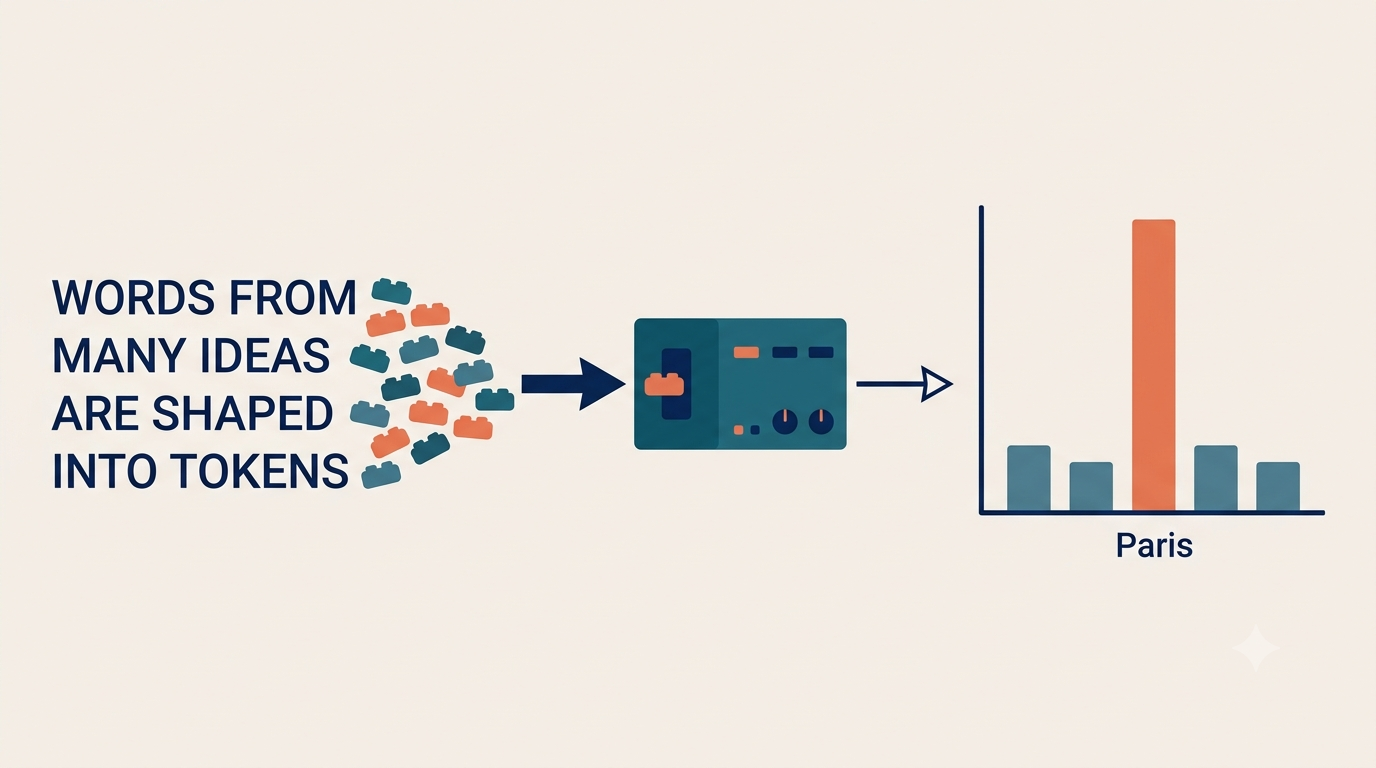
How an LLM Builds a Word

Part 1 of the series “From Token to Chatbot” — a hands-on journey from the inner mechanics of an LLM all the way to building your own chatbot.

An LLM (Large Language Model) feels magical: it writes, codes, translates, reasons. In this article, you’ll discover that it really does just one thing — and repeats it. By the end, you’ll have seen with your own eyes, in your terminal, a real model “hesitate” between several words and pick one. That moment is where the magic becomes understandable mechanics. Everything else in the series (attention, prompts, APIs, chatbot) builds on what you learn here.

📌 Who this is for: you’re comfortable with Python, but a complete beginner on LLMs. No machine learning knowledge is assumed. We move in very small steps, every notion is defined the first time it appears, and everything runs locally and for free (APIs come later in the series).

💻 Hardware prerequisites: the core hands-on parts run on CPU on any recent computer — GPT-2 is tiny, a GPU wouldn’t help. An optional Part D bonus taps a CUDA-capable NVIDIA GPU (ideally 8 GB of VRAM or more) to run a real modern model via Hugging Face. So you have nothing to enable for the basics; the GPU only comes into play in the bonus, and the whole core of the article works fine without it.

⏱️ Duration: plan for 2 to 3 hours, no rush. Better to do each hands-on step and understand it than to read everything fast. You can stop after Part B (the core) and keep Parts C and D for a second session.

---

🎯 Learning objectives

By the end of this article, you’ll be able to:

1. State in one sentence the single operation every LLM repeats.
2. Explain what a token is and why we don’t count in words or letters.
3. Read a model’s actual output (the next-word probabilities) and interpret it.
4. Write yourself the small loop that turns “one word” into “a sentence”.
5. Tell apart a deterministic answer from a varied one, and know where the difference comes from.

🧠 Keep these 5 objectives in mind. At the very end, you’ll tick them off one by one.

---

🧭 Prerequisites and setup

What you need to know: how to run a Python script. That’s it.

The tool we use throughout: uv. uv is a modern (blazing-fast) Python project and package manager. It replaces pip + venv: it creates an isolated environment for you, tracks your dependencies in a pyproject.toml file, and runs your scripts in the right environment. Every command in this series goes through uv — a good habit that prepares the real project (the chatbot that closes the series).

Step 0 — install uv (once per machine)

# macOS / Linux
curl -LsSf https://astral.sh/uv/install.sh | sh

# Windows (PowerShell)
powershell -ExecutionPolicy ByPass -c "irm https://astral.sh/uv/install.ps1 | iex"

Close and reopen your terminal, then check:

uv --version

✅ Checkpoint: a line like uv 0.x.y appears. If the command isn’t found, see ”🔧 If the install gets stuck” at the bottom.

Step 1 — create the project

We create a single project that will serve the whole journey. uv manages an isolated Python environment inside it automatically.

uv init llm-formation        # creates the project folder (with pyproject.toml)
cd llm-formation             # move into it: ALL following commands run from here

📌 Remember: from here on, you always work from the llm-formation/ folder. uv handles the isolated environment — you have nothing to activate or configure by hand.

Step 2 — add the first dependency

We go in two steps to avoid trouble. We start with the lightest one; we’ll add the heavier ones when we actually need them (Part B). That way, if something breaks, you’ll know exactly which step is to blame.

uv add tiktoken              # adds the dependency to the project (tracked in pyproject.toml)

💡 How we’ll run scripts: with uv run, which executes your script in the project environment (with the right dependencies), without you having to activate anything. For example uv run manip1.py. We create our files manip1.py, manip2.py… inside the llm-formation/ folder; you’ll come back to them in the episode on generation settings.

⚠️ Before complaining about an error: a full troubleshooting section awaits at the very bottom (”🔧 If the install gets stuck”). The first PyTorch download (Part B) is heavy (several hundred MB) and that’s normal. More on that when we get there.

---

🗺️ Overview: the one idea of the day

If you only remember one sentence today, make it this one:

📌 Key point: an LLM is a function that predicts the next word. It looks at the text so far, guesses the most plausible continuation, appends it, then starts over with the lengthened text. That’s all. “Reasoning”, code, translation: everything emerges from this loop repeated billions of times.

Here’s the full journey of a piece of text inside the model. Don’t try to understand everything now — this is the map of the trip, we’ll visit each stop:

   "The capital of France is"
              │
              ▼
   ┌──────────────────────┐   PART A
   │   1. TOKENIZATION     │   we split the text into small chunks ("tokens")
   └──────────────────────┘   and turn them into numbers
              │
              ▼
   ┌──────────────────────┐
   │   2. THE MODEL'S      │   the chunks are transformed and "talk to each other"
   │      BRAIN            │   (we'll open this box next episode — today
   └──────────────────────┘    we treat it as a black box)
              │
              ▼
   ┌──────────────────────┐   PART B  ← TODAY'S CORE
   │   3. ONE SCORE PER    │   the model scores EVERY possible word in the vocabulary
   │      POSSIBLE WORD    │   ("Paris" 87%, "the" 4%, "very" 0.1%, ...)
   └──────────────────────┘
              │
              ▼
   ┌──────────────────────┐
   │   4. WE PICK          │   we draw a word from this list of scores
   │      A WORD           │   → "Paris"
   └──────────────────────┘
              │
              └──────────►  we put "Paris" back at the end of the text, and START OVER
                            (that's what "generating a sentence" is)

📌 How to read this article: it’s split into four parts.

• Part A — text becomes numbers (the tokens).
• Part B — the model scores the words and picks one. This is the core, the eureka moment.
• Part C — to go one step further (optional on a first session).
• Part D — bonus: wake up your GPU with a real modern model (optional, recommended if you have an NVIDIA card).

🧵 Our through-line for the whole day: “Paris”

To never stay abstract, we follow a single example from start to finish. Our guinea pig: the sentence

“The capital of France is”

At each step, we look at what concretely happens to it. Final goal: watch a real model complete this sentence with “Paris”, and understand exactly how it gets there. Small challenge: keep this question in mind — at what precise moment does the model “decide” it’s Paris? The answer will surprise you.

---

---

PART A — Text becomes numbers

A computer only manipulates numbers. So the first mission is: turn text into numbers. It’s subtler than it looks, and it has very concrete consequences (right down to your bill when you use an API).

A.1 — The token: the real “chunk” the model sees

❓ Opening question (think for 10 seconds before reading on): in your view, does an LLM read letter by letter? word by word? And “hello” vs “Hello”: same or different to it?

The why: a necessary compromise

The model has to split any text into reusable chunks. Two simple ideas come to mind, and both fail:

• Split into letters? Sequences become huge (a paragraph = thousands of letters) and you lose the notion of a word.
• Split into whole words? You’d need a giant dictionary, and the model would choke on any rare, invented or misspelled word.

The chosen solution is a middle ground: the token. A token is a fragment of text — sometimes a whole word (“the”), sometimes part of a word, sometimes just a few characters. On average, a token ≈ 4 characters in English.

The analogy: LEGO bricks

You don’t build a house with plastic powder (letters: too fine) nor with pre-assembled houses (whole words: too rigid). You build with bricks of varying sizes. The most common bricks (the little 2×2) are ready to use; for rare shapes, you assemble several bricks. Same for text: a frequent word = one brick, a rare word = several bricks.

How the bricks are made (in short)

The method is called BPE (Byte-Pair Encoding). You don’t need to master its inner workings today, just the idea:

1. start from single characters;
2. merge the most frequent pair of characters/fragments in a huge corpus of text;
3. repeat tens of thousands of times, until you get a “vocabulary” of tokens (often ~100,000).

Consequence: it’s not grammar, it’s statistics. The most common fragments in text become unique tokens.

🔬 Hands-on 1 — see the tokens with your own eyes

Create manip1.py:

# manip1.py — observe how text is split into tokens
import tiktoken

# We load the "splitter" (tokenizer) used by the GPT-3.5 / GPT-4 family
enc = tiktoken.get_encoding("cl100k_base")

words = ["the", "transformer", "antidisestablishmentarianism", "GPT", " leading_space"]
for word in words:
    ids = enc.encode(word)                       # text  -> list of numbers (token IDs)
    chunks = [enc.decode([i]) for i in ids]      # decode each number on its own
    print(f"{word!r:30} -> {len(ids)} token(s): {chunks}")

Run it (from the llm-formation/ folder): uv run manip1.py

✅ Checkpoint — you should see something like:

• "the" → 1 token
• "transformer" → 1 or 2 tokens
• "antidisestablishmentarianism" → several tokens (a rare word → fragmented)
• " leading_space" → look closely: the space is glued to the first chunk!

If you see this, you’ve got the essentials: frequent words fit in one token, rare words break into several, and spaces are part of the tokens.

Three consequences you’ll really run into

📌 Key point:

1. You’re billed per token (input + output), never per word or character. Your future API bill depends on the number of tokens.
2. The context window (everything the model can “see” at once) is measured in tokens (e.g. “200,000 tokens”).
3. Non-English text often costs more than English: less present in training corpora, it fragments into more tokens to say the same thing.

The painful counter-example: counting characters

Many beginners estimate a cost or a size by counting characters. Bad idea:

# Add this at the end of manip1.py
text = "antidisestablishmentarianism " * 100
print("\nNumber of characters:", len(text))               # looks "small"
print("Number of TOKENS    :", len(enc.encode(text)))     # much higher

The character count systematically underestimates the cost for text rich in rare words or non-English. Always reason in tokens.

🧵 “Paris” — step 1: our sentence enters the machine

# Add this at the end of manip1.py
sentence = "The capital of France is"
ids = enc.encode(sentence)
print("\nOur through-line:")
print("  IDs   :", ids)
print("  Tokens:", [enc.decode([i]) for i in ids])
# Expected: ['The', ' capital', ' of', ' France', ' is']  -> 5 tokens (spaces included)

Remember this well: it’s this list of numbers, not the sentence, that enters the model. The model will never see “France”, it will see the number of the token France.

✍️ Your turn

1. In your own words: why is a token neither a letter nor a word?
2. Predict before testing: will “cat” and “cats” give the same token? Check with enc.encode.
3. Encode "Paris" then " Paris" (with a leading space). Same numbers or different? Why is this useful to know when you write a prompt?

👉 See the answers

1. The token is a statistical compromise. Letters would give endless sequences and lose word meaning; whole words would require a giant dictionary and fail on any rare or unknown word. The token captures the most frequent fragments of text, with a variable size.
2. Different. “cats” is often a distinct token, or else “cat” + “s”. The model doesn’t “know” by a rule that it’s a plural: it learned it statistically. Any variation (capitalization, plural, accent) can change the split.
3. Different numbers: the leading space is part of the token, so "Paris" ≠ " Paris". This matters because the way you join or space words in a prompt literally changes what the model receives. A small formatting detail can therefore influence the answer.

Mini-summary of A.1

• The model sees tokens (fragments of about 4 characters), not letters or words.
• Frequent words = 1 token; rare words = several. Spaces and capitalization count.
• We count, bill and measure context in tokens — never in characters.

---

A.2 — From number to “meaning”: the embedding (gently)

❓ Opening question: the token France became a number, say 6342. Can the model “think” with a serial number? What’s missing for a number to carry meaning?

The why: a number means nothing

The number 6342 is arbitrary. It isn’t “closer” to 6343 than to 12. If the model computed directly with these numbers, “France” and “Germany” would have no reason to be treated as close. So we need to replace each number with something rich and comparable.

That something is the embedding: a list of numbers (say 768 values) attached to each token. This list is the token’s “numeric ID card”.

The analogy: a map of meaning

Imagine a huge geographic map, but of words. Each word is a point on it. On this map, “king” and “queen” are neighbors; “king” and “banana” are at opposite ends; “Paris”, “London” and “Tokyo” form a small “capitals” district. A word’s coordinates on this map = its embedding.

💡 The idea to remember: turning a number into an embedding is placing the word on the map of meaning. And the genius is that these coordinates are learned: during training, the model placed the words all by itself so that close meanings end up close.

🔬 Hands-on 2 — “meaning becomes geometry”

This exercise has a single goal: make you feel that words close in meaning are close in distance. We use a small dedicated model (lightweight, free).

uv add sentence-transformers numpy

⚠️ This install is a bit heavier (it bundles PyTorch). First time = a few minutes, that’s normal. If it gets stuck, see ”🔧 If the install gets stuck” at the bottom.

# manip2.py — show that closeness in meaning = geometric closeness
from sentence_transformers import SentenceTransformer
import numpy as np

model = SentenceTransformer("all-MiniLM-L6-v2")   # small, free, runs locally

words = ["king", "queen", "man", "woman", "banana"]
vecs = model.encode(words)   # each word -> a list of numbers (its embedding)

def similarity(a, b):
    # cosine similarity: 1 = very close, 0 = unrelated
    return np.dot(a, b) / (np.linalg.norm(a) * np.linalg.norm(b))

print("king vs queen :", round(similarity(vecs[0], vecs[1]), 3))   # should be HIGH
print("king vs banana:", round(similarity(vecs[0], vecs[4]), 3))   # should be LOW

✅ Checkpoint: king vs queen should give a clearly larger number than king vs banana. If so: you just measured meaning with a distance. Words are no longer labels, they’re positions, and the position encodes the meaning.

⚠️ Common pitfall — an honest nuance: this small model produces one embedding per whole sentence, already “contextualized”. In a real LLM, the starting embedding is per token and not yet contextualized: at this stage, the tokens haven’t “talked” to each other yet. That’s exactly the job of the “model’s brain” (next episode) — to circulate context. What to keep today: the intuition “meaning = position on a map”. The exact mechanics come later.

🧵 “Paris” — step 2

Our 5 tokens (The, capital, of, France, is) each become a list of numbers. At this precise moment, the vector for France “knows” the general meaning of France, but doesn’t yet know we care about its capital. No token has talked to another yet. Hold on to that frustration: it’s exactly what the next episode will resolve.

✍️ Your turn

1. Why can’t we feed a token’s raw number (e.g. 6342) into the model’s computations?
2. Add "Paris" and "Tokyo" to the list in manip2.py. Compare similarity("king","Paris") and similarity("Paris","Tokyo"). What do you observe, and why?

👉 See the answers

1. Because a token number is arbitrary: its value reflects no similarity of meaning. The embedding replaces it with a learned list of numbers where closeness reflects similarity of meaning or usage — which makes the model’s computations meaningful.
2. “Paris” and “Tokyo” (two capitals) should be closer to each other than “king” and “Paris”. The model observed that city names appear in similar contexts, so it placed them in the same “district” of the map.

Mini-summary of A.2

• An embedding replaces a token’s number with a list of numbers: its position on the “map of meaning”.
• These positions are learned; closeness on the map ≈ closeness in meaning.
• At the start, tokens haven’t “talked” to each other yet: that’s the next episode’s job.

---

---

PART B — The model scores the words and picks one (THE CORE)

This is where it all happens. You’ll see the real output of a real model, and write the loop that builds a sentence yourself. If you do only one thing today, do this part.

B.1 — Install what’s needed (and understand what we’re installing)

We’ll load a real (small) LLM called GPT-2. It’s old and limited, but it’s perfect for learning the mechanics: it’s small, free, and runs instantly on your CPU. No need to mobilize a GPU here — GPT-2 is too small for it to make any difference. We’ll save the card for the Part D bonus.

uv add transformers torch

⚠️ This is the heaviest install of the day (torch weighs several hundred MB). The first time, it can take several minutes and seem frozen: that’s normal, let it run. If there’s trouble → ”🔧 If the install gets stuck” section. And if you really can’t install it, don’t drop out: Part B has a plan B without PyTorch below.

💡 CPU vs GPU, put simply: the CPU does few computations at a time but each very fast; the GPU does thousands in parallel. Big models love the GPU (lots of number-list multiplications at once). GPT-2 is so small that the CPU is plenty. We’ll see the difference concretely in Part D, where your GPU runs a much bigger model. The uv add torch command above installs, by default, a version that works on CPU — perfect for Parts B and C. The GPU (CUDA) version will be installed in Part D, when it actually matters.

Two words on what we’re installing:

• transformers (from Hugging Face): a library that downloads and runs ready-made models.
• torch (PyTorch): the “calculator” that does the operations on number lists. You don’t need to master it; we’ll use just a handful of functions, and I explain each one.

B.2 — A model’s real output: a score for EVERY word

❓ Opening question: at the very end, what does the model produce exactly? A word? A sentence? Think before reading.

The why: the model doesn’t pick a word, it scores every word

Here’s the most counter-intuitive idea of the day, so let’s take it slowly. When the model has to guess the continuation, it doesn’t “output” a word. It assigns a score to every possible token in its whole vocabulary (tens of thousands of tokens). For “The capital of France is”, it gives a big score to “Paris”, a small one to “the”, a tiny one to “banana”, etc.

These raw scores have a name: the logits. A score can be negative, or very large. They are not percentages yet.

The analogy: the jury that scores everyone

Imagine a jury facing 50,000 candidates (the vocabulary). Each candidate gets a raw score: those are the logits. Then an organizer converts all these scores into percentage chances that total 100%. This conversion has a fancy name — the softmax — but its role is simple: turn raw scores into comparable percentages.

📌 The two words to remember:

• logits = the model’s raw scores (one per possible word), from −∞ to +∞.
• softmax = the machine that turns these scores into probabilities (all positive, total = 100%). Important: softmax doesn’t change the ranking — the top-scored word stays the most probable.

🔬 Hands-on 3 — THE eureka moment: watch the model hesitate

This is the most important exercise so far. We’ll display the 10 words GPT-2 thinks of most to complete our sentence. I comment every line, especially those with tensors (don’t skip the comments):

# manip3.py — display the most probable words according to a real model
from transformers import GPT2LMHeadModel, GPT2Tokenizer
import torch

# 1) Load the splitter and the GPT-2 model (downloaded once, then cached)
tok = GPT2Tokenizer.from_pretrained("gpt2")
model = GPT2LMHeadModel.from_pretrained("gpt2")
model.eval()   # "evaluation" mode: we use the model, we don't train it

# 2) Our through-line, turned into token numbers
prompt = "The capital of France is"
ids = tok.encode(prompt, return_tensors="pt")
#   return_tensors="pt": returns a "PyTorch tensor" (an array of numbers
#   in the format the model expects), rather than a plain Python list.

# 3) Pass the tokens through the model
with torch.no_grad():           # "no_grad" = we don't compute training gradients
    output = model(ids)         #            -> faster, less memory
logits = output.logits
#   logits has 3 dimensions: [1, prompt_length, vocabulary_size]
#   - 1            : we sent 1 single sentence
#   - length       : one set of scores AFTER each token of the prompt
#   - vocabulary   : one score for EVERY possible word (~50,000 for GPT-2)

# 4) We only want to predict the NEXT word -> take the last set of scores
next_word_scores = logits[0, -1, :]
#   [0,  -1,  :] reads: "sentence #0 , LAST position , all the scores"
#   -1 = the last element (like in plain Python). That's the key: the score
#   placed right AFTER the prompt's last word is the prediction of the continuation.

# 5) Turn the raw scores (logits) into percentages (softmax)
probs = torch.softmax(next_word_scores, dim=-1)

# 6) Display the 10 top-scored words
top = torch.topk(probs, 10)    # gets the 10 highest values + their position
print(f"Prompt: {prompt!r}\n")
print("The model thinks the next word is probably:")
for prob, position in zip(top.values, top.indices):
    word = tok.decode([position])              # translate the number back to text
    print(f"   {word!r:12}  {prob.item()*100:5.2f} %")

Run it: uv run manip3.py (the first time, GPT-2 downloads — ~500 MB, be patient).

✅ Checkpoint — this is where the magic drops: you should see a list where “Paris” comes out on top (often 15-40%), followed by variants (“the”, “now”, “a”…). You’re literally watching a model hesitate, then lean toward Paris. That’s what’s under ChatGPT’s hood, in miniature. Take a second to savor it: you just opened the black box.

💡 Why English?: we picked an English sentence because GPT-2 was mostly trained on English — it’s much better at it. Try a non-English version, e.g. “La capitale de la France est”, and compare: the predictions will likely be less sharp. That concretely illustrates the language bias seen in Part A.

🧪 Plan B — without PyTorch (if the install failed)

If you couldn’t install torch, don’t get stuck. You can live the same idea with a pure-Python simulator: we invent raw scores and apply softmax by hand to see the scores → percentages conversion.

# manip3_planB.py — understand logits -> softmax WITHOUT any model
import math

# Suppose the model assigns these raw scores (logits) to 4 words:
words  = ["Paris", "the", "France", "banana"]
logits = [ 8.0,     5.0,   4.0,      -2.0   ]   # "Paris" is the top score

# Softmax, step by step:
exps  = [math.exp(x) for x in logits]   # apply the exponential to each score
total = sum(exps)                       # sum them all
probs = [e / total for e in exps]       # each score becomes a share of the total (=100%)

for word, p in zip(words, probs):
    print(f"   {word:8} {p*100:6.2f} %")
print("   (sum:", round(sum(probs)*100), "%)")

✅ Checkpoint plan B: run it with uv run manip3_planB.py. “Paris” comes out clearly on top, and the sum is 100%. You reproduced by hand what the end of every LLM does. Change the logits and observe: raise the score of “France” and watch its percentage climb.

💡 manip3_planB.py only uses the math module (shipped with Python), so no dependency to add: uv run executes it as-is in the project environment.

The counter-example: an open sentence

Take manip3.py again and replace the prompt with something vague:

prompt = "I think that"

✅ Observe: the list becomes flat — no word dominates, many have similar percentages. Compare with “The capital of France is” where one word crushed the others.

📌 The lesson: the shape of the list reflects the model’s uncertainty. Obvious continuation → “peaky” list (a clear winner). Open continuation → “flat” list (lots of tied candidates).

🧵 “Paris” — step 3: the answer to our challenge

Remember the opening question: at what moment does the model “decide” it’s Paris? Answer: it never really decides. It simply computed that, statistically, “Paris” is the most plausible token to continue this text, and gave it the highest score. No understanding, no decision: a plausibility computation. It’s unsettling, and yet that’s the whole secret.

✍️ Your turn

1. What’s the difference between a logit and a probability? What does the softmax do between the two?
2. The model gives logits [2.0, 1.0, 0.1] to three words. Without a calculator: which is most probable after softmax, and can softmax change that ranking?
3. Run manip3.py with the prompt "The sun rises in the". Does the expected word dominate? Is the list peaky or flat? Why?

👉 See the answers

1. A logit is a raw score (from −∞ to +∞) the model assigns to a word; it’s not directly interpretable. A probability is that score converted into a percentage (positive, and all together = 100%). The softmax is the operation that does this conversion, without changing the ranking of the words.
2. The first (logit 2.0) is most probable. Softmax always preserves the order: it only turns scores into percentages. It even widens the gap (via the exponential), so 2.0 gets a clearly larger share than 1.0 and 0.1.
3. “sun” should strongly steer toward “sky”: the list will be rather peaky (a clear winner), because the continuation of “The sun rises in the” is almost determined. A very predictable sentence concentrates the probability on few words.

Mini-summary of B.2

• A model’s real output = one score (logit) per word in its vocabulary.
• The softmax converts these scores into probabilities (total 100%) without changing the ranking.
• Peaky list = obvious continuation; flat list = open/uncertain continuation.

---

B.3 — From one word to a sentence: the loop (autoregression)

❓ Opening question: the model produces only one word at a time. But a ChatGPT answer is dozens of words. How do we go from one word to a whole sentence?

The why: we start over, again and again

One pass through the model predicts only one word. To make a sentence, we repeat: we append the chosen word to the end of the text, feed the whole thing back into the model, get the next word, and so on. This process has a name: autoregressive generation (“auto” = from its own output).

The analogy: autocomplete on steroids

It’s exactly your phone keyboard’s word suggestion, but on an automatic loop. You type a word, the keyboard suggests the next; here, the model accepts its own suggestion by itself and continues, again and again, without stopping.

🔬 Hands-on 4 — write generate() yourself in 6 lines

Libraries offer a ready-made model.generate() function. But to understand, we’ll rewrite it by hand. Reuse tok and model from hands-on 3:

# manip4.py — build a sentence by repeating the prediction
from transformers import GPT2LMHeadModel, GPT2Tokenizer
import torch

tok = GPT2Tokenizer.from_pretrained("gpt2")
model = GPT2LMHeadModel.from_pretrained("gpt2")
model.eval()

text = tok.encode("The capital of France is", return_tensors="pt")

for _ in range(15):                      # we'll produce 15 words, one by one
    with torch.no_grad():
        logits = model(text).logits      # scores for each position
    next_scores = logits[0, -1, :]       # keep the NEXT word's scores
    next_token = torch.argmax(next_scores)     # take the TOP-scored word
    next_token = next_token.view(1, 1)         # back to the right shape (array)
    text = torch.cat([text, next_token], dim=1)  # APPEND it to the end of the text

print(tok.decode(text[0]))   # translate the whole sequence back to text

Run it: uv run manip4.py. You just rewrote generate()!

✅ Checkpoint: you get a sentence starting with “The capital of France is Paris…” that continues. The key function is argmax: it always takes the top-scored word. That’s the so-called greedy strategy.

The counter-example: why ChatGPT, itself, varies

argmax is deterministic: same starting sentence → exactly the same output, every run. Re-run manip4.py several times to check: identical.

But ChatGPT gives you different answers to the same question. Why? Because in practice, we don’t always take the top score: we draw at random among the good candidates, respecting their percentages (sometimes #1, sometimes #2…). Replacing argmax with a weighted draw is exactly the subject of the next episode (the temperature and top-p settings).

💡 A revealing little experiment: with the prompt "Once upon a time", generate 40 words (range(40)) keeping argmax. You’ll often see the text go in circles or repeat. This “always the best” flaw is precisely what the next episode’s random draw fixes.

🧵 “Paris” — resolution

Loop complete. We: split “The capital of France is” into tokens (A.1) → turned each into a position on the map of meaning (A.2) → let (next episode) the model’s brain circulate the information → got one score per word, converted into percentages by softmax (B.2) → picked “Paris”, then started over for the next word (B.3). That’s the entirety of what an LLM does. Everything else in the series is about steering this loop intelligently.

✍️ Your turn

1. Explain “autoregressive” in your own words, to someone who knows nothing about it.
2. Why does the greedy strategy (argmax) always give the same output for a given prompt?
3. From what you saw, where does the variety in ChatGPT’s answers come from — a model being “creative”, or the way we pick the word?

👉 See the answers

1. Autoregressive = the model generates one word at a time, and each new word is computed from all the preceding text, including the words it just produced itself. It feeds on its own output to move forward, like an autocomplete chaining itself along.
2. Because argmax always chooses the highest-scored word, with no randomness. For the same prompt and the same model, the computed scores are identical every time, so the chosen word is too: the output is strictly reproducible.
3. From the way we pick the word. The model always produces the same list of scores; the variety comes from drawing at random among the good candidates instead of always taking #1. It’s not a model “creativity”, it’s a sampling choice (next episode).

Mini-summary of B.3

• Generating a sentence = repeating the prediction by re-injecting each produced word (autoregression).
• argmax (greedy) always takes the top score → deterministic, but tends to repeat.
• The variety of real answers comes from the weighted random draw → next episode.

---

---

PART C — To go one step further (optional)

You can stop here for today and keep this part for a second session. It adds two useful but non-essential notions to the core token → prob → loop.

C.1 — Why word order matters (position)

❓ Opening question: “the cat eats the mouse” and “the mouse eats the cat” use the same tokens. How does the model avoid confusing them?

Embeddings (A.2) say which word, but not where. Yet position changes the whole meaning. So the model adds, in each vector, a position information (a label “I’m the 1st word”, “I’m the 3rd”…).

The analogy: a recipe whose words were all dumped into a bag. You have the ingredients, but you’ve lost the order of the steps. Position information restores the order.

Recent models (like Llama) use an efficient method called RoPE (Rotary Position Embedding). The detail belongs to the next episode; today, just remember: word order is properly encoded, so the model tells the cat-eater from the eaten-mouse.

Mini-summary: without position information, word order would be lost. So we inject it into each vector (recent method: RoPE).

C.2 — The numbers that “make the size” of a model

When you read “7B” or “70B” model, it’s the number of parameters (the internal learned settings): 7 or 70 billion. Four numbers largely describe a model:

Number	What it is	Typical order of magnitude
vocabulary size	number of distinct tokens	~50,000 to ~130,000
vector dimension	length of the number list per token	768 to 4096+
number of layers	stacked floors in the “brain”	12 to 80+
context window	max tokens seen at once	1,000 to 1,000,000+

📌 Key point on the context window: when a conversation exceeds this limit, the model loses access to the beginning — the first tokens fall out of the window and are “forgotten”. That’s why a very long exchange can see the model lose the thread of what was said at the very start. The GPT-2 in your exercises has a small window (1024) and few parameters: hence its sometimes shaky answers.

Mini-summary: “7B” = 7 billion parameters. Four numbers describe a model; exceeding the context window = beginning of the conversation forgotten.

---

---

PART D — Bonus: wake up your GPU (optional, but recommended)

Up to now everything ran on CPU with GPT-2, a 2019 model. If you have a CUDA-capable NVIDIA GPU, you can shift up a gear. In this part, we’ll (1) install the GPU version of PyTorch cleanly with uv, (2) load a real modern model (2024) on it, and (3) compare its predictions to GPT-2’s. Goal: feel the gap between a small old model and a recent one, and watch your card fill up. It’s the day’s satisfying moment.

No NVIDIA GPU? No worries: you can skip this part without losing any of the article’s core. The “predict the next token” principle stays exactly the same.

D.1 — Install the GPU (CUDA) version of PyTorch with uv

The torch installed in Part B runs on CPU. To use your NVIDIA card, you need the CUDA version (NVIDIA’s GPU-computing technology). With uv, we point to PyTorch’s GPU package index.

Step 1 — check your card is seen by the system. Make sure a recent NVIDIA driver is installed, then check:

nvidia-smi

✅ Checkpoint: a table appears with your NVIDIA card’s name and a “CUDA Version: …” line. If the command doesn’t exist, your driver isn’t in place (see troubleshooting).

Step 2 — replace torch with its CUDA version in the project. We tell uv to fetch torch from PyTorch’s CUDA index (here CUDA 12.4; choose a version compatible with your driver):

uv add torch --index pytorch-cuda=https://download.pytorch.org/whl/cu124

⚠️ This download is heavier than the CPU version (the CUDA build bundles the GPU libraries). Expect some patience the first time. If uv complains about the index or version, the troubleshooting section covers the variants.

Step 3 — confirm PyTorch sees the GPU. Create manip5_gpu_check.py:

# manip5_gpu_check.py — does PyTorch see your NVIDIA card?
import torch

print("CUDA available:", torch.cuda.is_available())
if torch.cuda.is_available():
    print("Card detected :", torch.cuda.get_device_name(0))
    print("Total VRAM    :", round(torch.cuda.get_device_properties(0).total_memory / 1e9, 1), "GB")

Run: uv run manip5_gpu_check.py

✅ Decisive checkpoint: you should read CUDA available: True and your NVIDIA card’s name. If it’s True, you can put any model on your card. If it’s False, see the GPU troubleshooting — don’t move on until it’s True.

D.2 — The device reflex: run a model on GPU

Putting a model on GPU boils down to one idea: define a device (“cuda” if available, else “cpu”) and send the model and data to it with .to(device). It’s the reflex you’ll reuse throughout.

import torch
device = "cuda" if torch.cuda.is_available() else "cpu"   # pick GPU if possible
# ... then: model.to(device)   and   inputs.to(device)

💡 Why this little if? So that the same script runs everywhere: on a machine with an NVIDIA card it takes the GPU, on a machine without one it falls back to CPU without breaking. It’s a good portability habit.

D.3 — Load a real modern model (2024) on your card

We’ll load Qwen2.5-1.5B-Instruct: a model of ~1.5 billion parameters (≈ 20× GPT-2), recent, multilingual, that fits comfortably in 8 GB of VRAM. “Instruct” means it was trained to follow instructions (unlike GPT-2, which only continues text) — you’ll see the difference.

Create manip6_modern_model.py:

# manip6_modern_model.py — a real recent model on your GPU
from transformers import AutoModelForCausalLM, AutoTokenizer
import torch

device = "cuda" if torch.cuda.is_available() else "cpu"
name = "Qwen/Qwen2.5-1.5B-Instruct"

# AutoTokenizer / AutoModelForCausalLM: "generic" versions that automatically
# load the right model type from its name (handy: one piece of code for
# different models).
tok = AutoTokenizer.from_pretrained(name)
model = AutoModelForCausalLM.from_pretrained(
    name,
    torch_dtype=torch.float16,   # 16-bit numbers = 2× less VRAM, ideal on 8 GB
).to(device)                     # WE SEND THE MODEL TO THE GPU

# "Instruct" models expect a conversation format (user/assistant roles).
# apply_chat_template puts our question in the exact format the model expects.
messages = [{"role": "user", "content": "Explain in one sentence what a token is, for a beginner."}]
inp = tok.apply_chat_template(messages, add_generation_prompt=True, return_tensors="pt").to(device)

# Generate an answer (here we let generate() run the loop we wrote in manip4).
with torch.no_grad():
    output = model.generate(inp, max_new_tokens=80, do_sample=False)

# Only display the tokens ADDED by the model (we strip the original question).
answer = tok.decode(output[0][inp.shape[1]:], skip_special_tokens=True)
print(answer)

Run: uv run manip6_modern_model.py (first time: ~3 GB download, be patient).

✅ Checkpoint: you get a real, clean, relevant explanation. Mentally compare with GPT-2 (hands-on 3-4) which often went off into repetitions or gibberish. Same mechanics under the hood — next-token prediction — but 20× more parameters and modern training: the result is worlds apart.

Watch your card while it runs. Open a second terminal and run:

watch -n 1 nvidia-smi

✅ Visual checkpoint: during loading then generation, the “Memory-Usage” column climbs (the model takes ~3-4 GB of VRAM), and GPU usage (“GPU-Util”) rises during generation. You literally see your card working.

D.4 — The comparison that anchors it all: GPT-2 vs Qwen on the SAME exercise

Take the founding exercise (next-word probabilities, hands-on 3) but on the modern model, to compare the sharpness of the predictions. We keep our through-line.

# manip7_comparison.py — "the capital of France is" seen by a modern model
from transformers import AutoModelForCausalLM, AutoTokenizer
import torch

device = "cuda" if torch.cuda.is_available() else "cpu"
name = "Qwen/Qwen2.5-1.5B-Instruct"
tok = AutoTokenizer.from_pretrained(name)
model = AutoModelForCausalLM.from_pretrained(name, torch_dtype=torch.float16).to(device)
model.eval()

prompt = "The capital of France is"
ids = tok.encode(prompt, return_tensors="pt").to(device)   # data ALSO on the GPU

with torch.no_grad():
    logits = model(ids).logits

probs = torch.softmax(logits[0, -1, :], dim=-1)
top = torch.topk(probs, 10)
print(f"Prompt: {prompt!r}\nTop 10 according to Qwen2.5-1.5B:")
for prob, position in zip(top.values, top.indices):
    print(f"   {tok.decode([position])!r:12}  {prob.item()*100:5.2f} %")

Run: uv run manip7_comparison.py

✅ Comparative checkpoint: “Paris” should dominate even more clearly than in GPT-2 (higher probability, weaker competitors). A more capable model is more sure of the right answer on a simple fact. You observe the same probability distribution as in B.2 — but sharper. That’s what “a better model” means.

📌 The lesson of Part D: nothing magical changed. Still tokens, embeddings, logits, a softmax, a loop. What changes between 2019 and 2024 is scale (20× more parameters), training (instruction following), and the hardware that makes it all smooth. The day’s mechanics stay exactly the same — they just scale up.

✍️ Your turn

1. What is the line device = "cuda" if torch.cuda.is_available() else "cpu" for, and why is it a good habit?
2. Why do we load the model in torch.float16 rather than full precision, on an 8 GB card?
3. Ask a real question in manip6 (change the content), e.g. “Give me 3 recipe ideas with eggs.” Could GPT-2 have answered as cleanly? Why?

👉 See the answers

1. It automatically picks the GPU if available, else the CPU. Good habit because the same script becomes portable: it uses your NVIDIA card here, but would still run on a card-less machine, unchanged.
2. float16 encodes each number on 16 bits instead of 32, which halves the VRAM the model occupies. On 8 GB, that’s what lets you comfortably load a 1.5-billion-parameter model (and aim for bigger ones). The precision loss is negligible for inference.
3. No. GPT-2 (2019) was not trained to follow instructions: it only continues text, so it would likely wander off. Qwen2.5-Instruct underwent specific training (instruction tuning) that teaches it to answer a request — hence a structured, relevant reply. Same prediction mechanics, different training.

Mini-summary of Part D

• The GPU (CUDA) version of PyTorch installs with uv add torch --index ...; check with torch.cuda.is_available().
• The device + .to(device) reflex sends model and data to the card (and stays portable).
• A modern model (Qwen2.5-1.5B) on a recent GPU gives answers beyond comparison with GPT-2 — same mechanics, higher scale and training.

---

---

⚠️ Common pitfalls (cross-cutting recap)

Pitfall	Why it’s dangerous	The right reflex
Counting characters to estimate cost/context	Strongly underestimates (especially non-English/rare words)	Count in tokens: len(enc.encode(text))
Believing "word" = " word"	The space is part of the token → different input	Mind the formatting of prompts
Confusing logit and probability	You reason wrong about what the model “thinks”	Logit = raw score; after softmax = percentage
Believing the model “understands” like a human	Wrong mental model → unrealistic expectations	Remind yourself: next-word prediction, full stop
Taking the MiniLM exercise for the exact mechanism of an LLM	Confuses sentence embedding and token embedding	Keep the intuition (meaning = position), nuance next episode
Believing ChatGPT’s variety comes from “creativity”	False understanding of randomness	It’s the random draw (next episode), not the model
Giving up on the first slow uv add torch	It’s heavy and slow: normal, not a failure	Be patient; else → troubleshooting section + plan B

---

🔁 Final synthetic recap

              AN LLM = PREDICT THE NEXT WORD, IN A LOOP
                                │
        ┌───────────────────────┼───────────────────────┐
        ▼                       ▼                       ▼
   PART A                   PART B                  PART C
 text -> numbers         scores -> choice         (optional)
        │                       │                       │
   ┌────┴────┐         ┌────────┴────────┐      ┌───────┴────────┐
 TOKENS   EMBEDDING   LOGITS  ->  PROBS   AUTO-  POSITION   SIZE
(LEGO     (meaning =  (1 score  (softmax, REGRES-(order     (4 numbers,
 bricks,   position    per word) total    SION   matters:   context
 spaces    on a                 100%)    (loop:  RoPE)      window)
 count)    map)                          we re-
                                         inject)

💻 Part D (GPU bonus): the same mechanics, scaled up on an NVIDIA card. The device = "cuda" + .to(device) reflex, model loaded in float16, and a modern model (Qwen2.5-1.5B) that crushes GPT-2 in quality — without changing the “predict the next token” principle at all.

🧠 Self-assessment (actually do it): without re-reading, can you (a) redraw the text → next word journey naming each step, and (b) explain to someone why argmax always gives the same answer while ChatGPT varies? If a step trips you up, go back to that section before the quiz.

---

✅ Validation quiz

1. State in one sentence the single operation every LLM repeats.
2. Why does non-English text often consume more tokens (thus cost more) than the same text in English?
3. What is an embedding, and what does “meaning becomes geometry” mean?
4. Difference between logits and probabilities — and what does the softmax do between the two?
5. Why is generation called autoregressive, and why does argmax (greedy) always produce the same output for a given prompt?

👉 See the answer key

1. An LLM predicts the next word (token) from the preceding text, then repeats the operation by re-injecting that word. Any apparent capability (reasoning, code, translation) emerges from this loop.
2. Because training corpora, and therefore tokenizers, are dominated by English: a common English word often fits in one token, while less-frequent languages fragment into several tokens. More tokens = more cost (per-token billing) and more context consumed.
3. An embedding is a list of numbers associated with a token, serving as its starting representation in the model. “Meaning becomes geometry” means these lists are learned so that words close in meaning/usage end up close in space: you can then measure a similarity of meaning by a distance.
4. Logits are the raw scores (from −∞ to +∞) assigned to each word of the vocabulary. Probabilities are obtained by passing these scores through the softmax, which makes them positive and summing to 100%, without changing their ranking. Softmax bridges “raw score → usable percentage”.
5. Autoregressive: the model generates one word at a time relying on its own output (all the text produced so far) to compute the next. argmax systematically chooses the top-scored word, with no randomness; for the same prompt and model, the scores are identical every time, so the output is strictly reproducible (deterministic).

🧠 Objectives check: go back to the 5 objectives from the start. For each, can you say “yes, I can do it”? If a single one resists, you know exactly which section to reread — that’s active learning.

---

🔧 If the install gets stuck (troubleshooting)

With uv, most classic beginner headaches (wrong Python, “managed” environment, forgotten activation) disappear: uv handles the isolated environment on its own. Here are the cases that remain.

“uv: command not found (or unknown command).” uv isn’t installed, or your terminal hasn’t picked it up yet. Close and reopen your terminal after installing (Step 0). If it persists, re-run the Step 0 install script and read the last line: it sometimes points to a folder to add to your PATH.

“uv add torch seems frozen / very long.” That’s normal: PyTorch weighs several hundred MB. uv is fast at resolving dependencies, but the download depends on your connection (count a few minutes). As long as there’s no red error message, it’s progressing.

“I no longer know if I’m in the right folder.” All uv add / uv run commands must be run from llm-formation/ (the folder created in Step 1). Check with pwd (macOS/Linux) or cd (Windows): the path must end with llm-formation. If needed, cd to that folder.

“ModuleNotFoundError: No module named 'torch' (or ‘transformers’).” With uv, this almost always signals one of two causes: either the dependency wasn’t added (re-run uv add torch), or you’re running the script without uv run (a plain python manip3.py doesn’t use the project environment). Always run with uv run manip3.py: uv then guarantees the right dependencies are there.

“The GPT-2 download fails / cuts off.” The first run downloads the model (~500 MB) from Hugging Face (this isn’t handled by uv, but by transformers). Just re-run uv run manip3.py: the download resumes and caches. Check your connection.

“Too slow / too heavy for my machine.” GPT-2 runs on CPU without trouble, but if it really stalls: use the plan B without PyTorch (uv run manip3_planB.py) to understand logits → softmax, and come back to the PyTorch exercises later. You don’t lose the concept.

“Yellow warnings appear.” Warnings are not errors. If the script produces its result, ignore them.

GPU / CUDA specific cases (Part D)

“nvidia-smi: command not found.” The NVIDIA driver isn’t (or is no longer) in place. Install it at the system level (on Ubuntu: sudo ubuntu-drivers autoinstall then reboot) — it’s independent of Python and uv.

“torch.cuda.is_available() returns False while nvidia-smi works.” This is the most common case: you installed the CPU torch (Part B), not the CUDA version. Redo Step 2 of Part D (uv add torch --index pytorch-cuda=...) to replace torch with its GPU build, then re-run manip5_gpu_check.py.

“uv rejects the CUDA index or version.” The CUDA version in the URL (cu124) must be compatible with your driver. The “CUDA Version” line of nvidia-smi shows the maximum supported version: as long as cu124 is less than or equal to it, you’re fine. If needed, try a lower version (cu121) by changing the end of the URL.

“CUDA out of memory.” The model doesn’t fit in your VRAM. Check you’re loading in torch_dtype=torch.float16 (and not full precision). Close other VRAM-hungry apps (heavy browser, games). As a last resort, take a smaller model (e.g. a 0.5B variant). 1.5B in float16 fits easily in 8 GB.

“The modern model download (~3 GB) cuts off.” Like GPT-2, it’s transformers downloading from Hugging Face, not uv. Re-run the script: it resumes and caches.

💡 General reflex: paste the exact error message into a search engine — 99% of beginner errors are already solved somewhere.

📌 Cheat sheet of the day’s uv commands:

• uv init llm-formation — create the project (once)
• uv add <package> — add a dependency (CPU by default)
• uv add torch --index pytorch-cuda=https://download.pytorch.org/whl/cu124 — GPU torch version (Part D)
• uv run <script>.py — run a script in the project environment
• uv --version — check uv is properly installed

---

🚀 Going further

🔄 Another angle (same topic, different approach)

Resource	Type	How the angle differs	Effort
3Blue1Brown — “But what is a GPT?” (YouTube)	Video	Everything explained via animated visualization rather than code: the perfect complement to today’s exercises	Watch (~25 min)
Tiktokenizer (tiktokenizer.vercel.app)	Web tool	See tokenization live, without writing code: “immediate manipulation” angle	Play with it
”The Illustrated Transformer” — Jay Alammar (jalammar.github.io)	Article	Explains the mechanics via step-by-step diagrams rather than formulas	Read

🧩 Complementary (broaden the scope)

Resource	Type	The concrete link with today	Effort
Hugging Face — NLP Course, “Tokenizers” chapter (huggingface.co/learn)	Free course	Deepens the BPE seen in Part A; direct basis for the upcoming APIs	Read + practice
OpenAI Tokenizer (platform.openai.com/tokenizer)	Web tool	Estimate tokens and cost before calling a paid API	Play with it
transformers docs — “Generation” (huggingface.co/docs)	Official docs	Extends hands-on 4: all the generate() settings we’ll see next episode	Read + practice
Hugging Face Hub — “text-generation” models (huggingface.co/models)	Catalog	Find other models that fit in 8 GB to replay Part D	Explore

🔬 Deep dive (dig into the topic itself)

Resource	Type	Level / prerequisites	Effort
Andrej Karpathy — “Let’s build the GPT Tokenizer” (YouTube)	Video	Intermediate; code BPE from scratch. Prereq: Python + Part A	Guided practice
Andrej Karpathy — “Let’s build GPT: from scratch” (YouTube + nanoGPT repo)	Video + code	Intermediate/advanced; builds a whole GPT. Prereq: PyTorch basics	Intensive practice
”Attention Is All You Need” (arxiv.org/abs/1706.03762)	Research paper	Advanced; the founding paper. Read after the next episode	Demanding read

---

➡️ Next episode — Attention: we open the one box we left closed today — the “model’s brain”, i.e. the layers and the famous attention mechanism. You’ll discover how the vector for France ends up “knowing” we’re talking about its capital — and thus how “Paris” climbs to the top of the scores. Come back with your exercises done and all your questions.