Attention: How Words Talk to Each Other

Part 2 of the series “From Token to Chatbot” — a hands-on journey from the inner mechanics of an LLM all the way to building your own chatbot.

In the previous episode, you discovered that an LLM does just one thing: predict the next token, over and over. But we left one box closed — the “model’s brain”. We stopped on a very specific frustration: the vector for France “knew” the general meaning of France, but didn’t yet know we cared about its capital, because no token had “talked” to another yet. Today, we open that box. You’ll discover the mechanism behind the whole AI revolution since 2017: attention.

📌 Who this is for: you’re coming out of the previous episode (tokens, embeddings, logits, softmax, the autoregressive loop). No machine learning knowledge is assumed. And above all: no math background is assumed either. This document was purpose-built so the math is never an obstacle: we start with a toolbox that builds, from scratch and with tiny numbers, the only three operations we’ll need. You’ll never meet a formula without first taming it by hand.

💻 Hardware prerequisites: the core hands-on parts run on CPU on any recent computer — we work with tiny examples to understand, a GPU wouldn’t help. A bonus Part D (optional) visualizes the attention of a real model; it benefits from a CUDA-capable NVIDIA GPU if you have one, but the model used (DistilBERT) is light enough to run on CPU too. We stay on uv and the llm-formation project created in the previous episode.

⏱️ Duration: plan for 3-4 h including the math toolbox (take your time). Attention is the key notion for everything that follows. Suggested split: Part 0 + A + B in session 1; C + D in session 2.

---

🎯 Learning objectives

By the end of this module, you’ll be able to:

1. Handle without friction the three math tools of attention: dot product, multiplying arrays of numbers, softmax.
2. Explain the problem attention solves (why the embeddings from the previous episode weren’t enough).
3. Define the three roles Query, Key, Value with a simple, jargon-free analogy.
4. Compute by hand an attention score between two words and say what it means.
5. Describe what multi-head and stacked layers add, and place attention inside a Transformer.

🧠 Keep these 5 objectives in mind. At the end, you’ll come back and tick them off one by one.

---

🧭 Prerequisites and setup

On the knowledge side: what you learned in the previous episode (above all: a token becomes an embedding, a list of numbers = a position on the “map of meaning”). Nothing else: the required math is taught right here, in Part 0.

On the tooling side: we reuse the llm-formation project from the first episode. Move into it:

cd llm-formation        # the uv project created in the previous episode

For the core parts (Parts 0 to C), we only need NumPy (often already there from the first episode):

uv add numpy            # if already added before, uv does nothing: that's normal

💡 uv command reminder: uv add <package> for a dependency, uv run <script>.py to run a script in the project’s environment.

⚠️ A troubleshooting section is waiting for you at the bottom (”🔧 If you get stuck”).

---

---

PART 0 — Math toolbox (read this first)

🧰 Why this part exists: attention rests entirely on three operations, and it’s those — not the idea of attention — that scare people off at first. So we’ll build them one by one, with small whole numbers we compute by hand, before seeing a single complicated line. Once these three tools are in your pocket, attention becomes easy. Don’t skip this part: it’s the investment that makes everything else simple.

The three tools:

1. The dot product — measure whether two lists of numbers “point the same way”.
2. Array multiplication (and the @, .T notation) — do many dot products at once.
3. Softmax — turn arbitrary scores into percentages that add up to 100%.

0.1 — Tool #1: the dot product

The idea in one sentence

📌 The dot product takes two lists of numbers of the same length, multiplies them term by term, and adds it all up. The result is a single number. That number is large when the two lists “look alike”, small (or negative) when they oppose each other.

The computation, by hand, with small numbers

Take two lists of 3 numbers: A = [2, 1, 0] and B = [3, 1, 4].

We line them up, multiply each pair, and add:

   A =  [ 2 ,  1 ,  0 ]
   B =  [ 3 ,  1 ,  4 ]
         │    │    │
         ▼    ▼    ▼
       2×3  1×1  0×4        (multiply each pair)
        6  + 1  + 0  = 7    (add it all up)

   Dot product of A and B = 7

That’s it. No subtlety: multiply the pairs, add.

Why it measures “resemblance”

Look at these three cases (compute them yourself for practice):

• [1, 0] and [1, 0] → 1×1 + 0×0 = 1 (identical → large)
• [1, 0] and [0, 1] → 1×0 + 0×1 = 0 (nothing in common → zero)
• [1, 0] and [-1, 0] → 1×(-1) + 0×0 = -1 (opposite → negative)

💡 The intuition to keep: two lists “pointing the same direction” give a large dot product; two “unrelated” lists give zero; two “opposite” lists give a negative number. It’s exactly the resemblance measure we used in the previous episode (“close meaning = close vectors”), in raw form.

🔬 Micro-exercise 0-A — the dot product in Python (two ways)

Create j2_p0_dot_product.py:

# j2_p0_dot_product.py — the dot product, by hand then with NumPy
import numpy as np

A = [2, 1, 0]
B = [3, 1, 4]

# --- Way 1: "by hand", with a loop (to really SEE what happens) ---
total = 0
for i in range(len(A)):
    product = A[i] * B[i]
    print(f"  {A[i]} × {B[i]} = {product}")
    total = total + product
print("Dot product (by hand) :", total)

# --- Way 2: with NumPy, in a single operation (the shortcut) ---
a = np.array(A)
b = np.array(B)
print("Dot product (NumPy)   :", a @ b)   # the @ symbol does exactly Way 1

Run it: uv run j2_p0_dot_product.py

✅ Checkpoint: both ways give 7. You just saw that the @ symbol in Python is nothing more than “multiply the pairs and add” — the loop you wrote above. Keep this: @ = an automated dot product.

📚 External resource (dot product, explained visually)

• 3Blue1Brown — “Dot products and duality” (chapter 9 of the Essence of Linear Algebra series), on youtube.com (3Blue1Brown channel) or 3blue1brown.com/lessons/dot-products. The best visual explanation: it shows geometrically why the dot product measures a resemblance of direction. Watch it if the intuition doesn’t feel obvious yet.
• More textbook-style written alternative: Khan Academy, search “dot product” (khanacademy.org). Lots of worked exercises.

Mini-summary 0.1: dot product = multiply term by term + add → one number that measures resemblance. In Python: a @ b.

0.2 — Tool #2: multiplying arrays (and the @, .T notation)

The why

In practice, we don’t do one dot product, but many at once: “word X compared to all the other words”. An array of numbers (a matrix) lets us stack several lists, and array multiplication computes all the dot products in a single operation.

An array = stacked rows

A matrix is just lists arranged in rows. For example, 3 words each having 2 numbers:

        column 0    column 1
row 0   [   1    ,     0    ]   ← word 0
row 1   [   0    ,     1    ]   ← word 1
row 2   [   2    ,     3    ]   ← word 2

We say this array has a shape of “3 rows × 2 columns”, written 3×2.

The rule of @ multiplication, in one picture

When we write M @ N, each cell of the result is the dot product of a row of M with a column of N. Take a tiny example, entirely by hand:

   M (2×2)          N (2×2)
   [1  2]           [5  6]
   [3  4]           [7  8]

   Result R = M @ N , cell by cell:

   R[0,0] = (row 0 of M) · (col 0 of N) = [1,2]·[5,7] = 1×5 + 2×7 = 19
   R[0,1] = (row 0 of M) · (col 1 of N) = [1,2]·[6,8] = 1×6 + 2×8 = 22
   R[1,0] = (row 1 of M) · (col 0 of N) = [3,4]·[5,7] = 3×5 + 4×7 = 43
   R[1,1] = (row 1 of M) · (col 1 of N) = [3,4]·[6,8] = 3×6 + 4×8 = 50

   R = [19  22]
       [43  50]

📌 The only thing to remember: @ between two arrays = many dot products (left row × right column), arranged in a grid. You already know how to do a dot product (0.1); @ just repeats it.

.T: “laying the array on its side” (transposition)

Sometimes, for the dot products to line up right, we need to swap the rows and columns of an array. That’s transposition, written .T. Visually, we tip the array onto its side:

   K (3×2)                K.T (2×3)   ← rows and columns swapped
   [1  0]                 [1  0  2]
   [0  1]        .T  →     [0  1  3]
   [2  3]

Row [1, 0] of K becomes column [1, 0] of K.T, and so on. We’ll use it for one simple reason: when we want to compare every row of one array with every row of another, we write A @ B.T. The .T puts the second array “the right way round” so each comparison is a row-against-row dot product.

💡 You don’t need to master the theory of transposition. Keep the usage: A @ B.T = compare every row of A with every row of B (all the cross dot products). That’s precisely what attention does.

🔬 Micro-exercise 0-B — check the multiplication by hand

Create j2_p0_matrix_mult.py:

# j2_p0_matrix_mult.py — checking @ and .T on small arrays
import numpy as np

M = np.array([[1, 2],
              [3, 4]])
N = np.array([[5, 6],
              [7, 8]])

print("M @ N =")
print(M @ N)          # should print [[19 22] [43 50]] — the numbers computed by hand

K = np.array([[1, 0],
              [0, 1],
              [2, 3]])
print("\nK (shape", K.shape, ") :")
print(K)
print("\nK.T (shape", K.T.shape, ") — rows and columns swapped:")
print(K.T)

# "Compare every row of K with every row of K" = K @ K.T
print("\nK @ K.T (all the cross dot products) :")
print(K @ K.T)

Run it: uv run j2_p0_matrix_mult.py

✅ Checkpoint: M @ N does give [[19 22] [43 50]] (your by-hand computations!), and you see .T swap rows and columns. Look at K @ K.T: it’s a 3×3 grid where cell (i, j) says how much word i resembles word j. This grid of resemblances is exactly what attention computes — you’re almost there.

📚 External resource (matrix multiplication, step by step)

• Khan Academy — “Multiplying matrices” (khanacademy.org, Precalculus › Matrices section). Short Sal Khan videos that redo the computation cell by cell, exactly like above, with auto-graded exercises. Ideal if the “row × column” rule doesn’t feel automatic yet.
• Picture + code version: Built In, “Dot Product of a Matrix: Explained” (builtin.com) shows the dot-product → matrix-multiplication link with NumPy screenshots.

Mini-summary 0.2: an array = stacked rows (shape “rows × columns”). @ = many dot products (row × column). .T = swap rows/columns. A @ B.T = all the cross resemblances.

0.3 — Tool #3: softmax

The why

We often get raw scores (arbitrary numbers, sometimes negative) and want to turn them into percentages: positive, and summing to 100%. That lets us read them as “shares” (weights). That’s the job of softmax — you already met it in the previous episode to go from logits to probabilities.

The recipe, in 3 moves

For a list of scores:

1. Exponential of each score. (The exponential, written exp, turns any number into a positive number; it crushes negatives toward 0 and makes positives climb fast — which amplifies the gaps.)
2. Add all these results → a total.
3. Divide each exponential by that total → each score becomes a share of the total. The sum is necessarily 100%.

The computation, by hand, with small numbers

Take three scores: [2, 1, 0].

   Step 1 — exponential of each score (rounded values):
      exp(2) ≈ 7.39
      exp(1) ≈ 2.72
      exp(0) = 1.00

   Step 2 — total:
      7.39 + 2.72 + 1.00 = 11.11

   Step 3 — each divided by the total:
      7.39 / 11.11 ≈ 0.665   → 66.5 %
      2.72 / 11.11 ≈ 0.245   → 24.5 %
      1.00 / 11.11 ≈ 0.090   →  9.0 %

   Sum: 66.5 + 24.5 + 9.0 = 100 %   ✅

📌 What to remember: softmax turns any scores into percentages summing to 100%, without changing their order (the largest score stays the largest percentage). It amplifies the gaps: here, a score of 2 vs 1 (a gap of 1) becomes 66% vs 24% (a much sharper gap). That’s what makes the winner “stand out”.

🔬 Micro-exercise 0-C — softmax in Python (by hand then the shortcut)

Create j2_p0_softmax.py:

# j2_p0_softmax.py — softmax, broken down then in short form
import numpy as np

scores = np.array([2.0, 1.0, 0.0])

# --- Broken-down version (the 3 moves, visible) ---
step1 = np.exp(scores)           # exponential of each score
print("Step 1 (exp)   :", np.round(step1, 2))
step2 = step1.sum()              # total
print("Step 2 (total) :", round(step2, 2))
step3 = step1 / step2            # each divided by the total
print("Step 3 (shares):", np.round(step3, 3))
print("Sum of shares  :", round(step3.sum(), 3), "(=1, i.e. 100 %)")

# --- Short, reusable version (a softmax function) ---
def softmax(x):
    e = np.exp(x - x.max())      # the "- x.max()" just avoids numbers that are too big
    return e / e.sum()           # (it doesn't change the result, it stabilizes it)

print("\nWith the softmax function:", np.round(softmax(scores), 3))

Run it: uv run j2_p0_softmax.py

✅ Checkpoint: you get roughly [0.665, 0.245, 0.090], sum = 1 — exactly your by-hand computations. The little softmax(x) function will serve you in every following exercise. (The - x.max() is a technical stability detail: it avoids gigantic exponentials, without changing the result.)

📚 External resource (softmax, simply)

• Video “Softmax function explained” on youtube.com (many short 5-8 min versions; search “softmax explained simply”). They visualize the 3 moves exp → sum → divide.
• Written: the page “Softmax activation function” on machinelearningmastery.com explains softmax’s role with accessible numerical examples.

Mini-summary 0.3: softmax = exp of each score, then each divided by the total → percentages summing to 100%, order preserved, gaps amplified.

---

🧰 End of the toolbox. You now hold the three tools attention needs: dot product (resemblance), @/.T multiplication (many resemblances at once), softmax (scores → shares). Everything that follows just combines them. If one of the three is still fuzzy, redo its micro-exercise and watch its resource before continuing — the rest depends directly on it.

---

---

🗺️ Big picture: the single idea of the episode

If you keep only one sentence about attention itself:

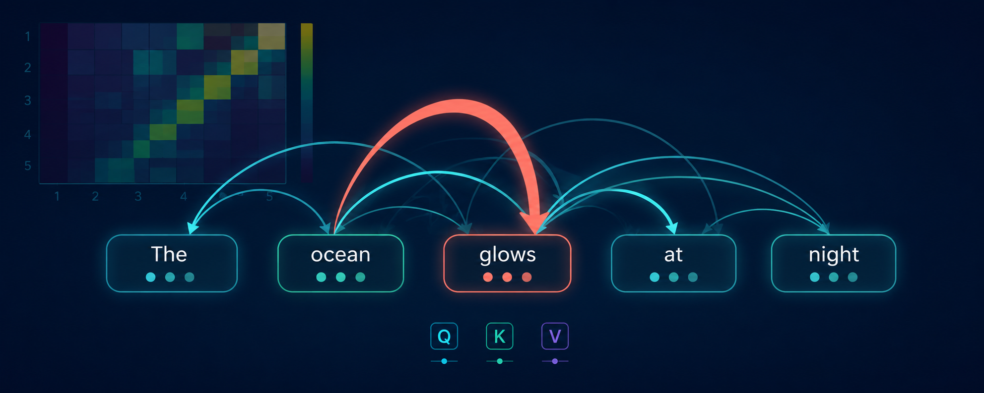
📌 Key point: attention lets each word look at the other words in the sentence and pull the useful information from them, to enrich its own meaning based on context. It’s the operation that turns a plain list of independent words into a sentence where each word “understands” its surroundings.

Let’s place it back in the pipeline from the previous episode, with the box we open today highlighted:

   "The capital of France is"
              │
              ▼
   [ TOKENIZATION ]        episode 1 — text split into tokens, then into numbers
              │
              ▼
   [ EMBEDDINGS ]          episode 1 — each token = a position on the map of meaning
              │            (BUT: the words haven't "talked" to each other yet)
              ▼
   ╔════════════════════╗
   ║  THE BRAIN:        ║   ◄────  THIS EPISODE, RIGHT HERE
   ║  stacked           ║         stacked layers, whose core is
   ║  Transformer       ║         the ATTENTION MECHANISM: words exchange
   ║  layers (ATTENTION)║         information and enrich one another
   ╚════════════════════╝
              │
              ▼
   [ LOGITS -> SOFTMAX ]   episode 1 — one score per possible word -> probabilities
              │
              ▼
   [ WE PICK A WORD ]      episode 1 -> "Paris", then we start over (autoregression)

📌 How to read what follows: four parts.

• Part A — why attention is necessary (the problem to solve).
• Part B — how attention works, combining your 3 tools. This is the core.
• Part C — what turns this brick into a real Transformer (multi-head, layers).
• Part D — bonus: visualizing the attention of a real model (on your GPU if you have one).

🧵 Our through-line (continued from the previous episode): “Paris”

In the previous episode, the vector for France didn’t “know” we were talking about a capital. Today’s question, solved in Part B:

How will the word is, at the moment of predicting the continuation, “look at” capital and France to understand that a capital name is expected — and thus push “Paris” up?

---

---

PART A — Why embeddings aren’t enough

Before learning how attention works, you need to feel why we need it. This part is short but conditions everything else. (It contains no math: breathe.)

A.1 — The problem of frozen meaning

❓ Opening question: does the word “bank” have a single meaning? If a model assigns a single fixed vector to “bank”, what happens in “I sat by the river bank” vs “I deposited cash at the bank”?

The observation

In the previous episode, each token receives an embedding — a position on the map of meaning. But that position is frozen: “bank” has the same starting vector regardless of context. Yet in “the river bank” it’s a shoreline, and in “the bank approved my loan” it’s a financial institution. A frozen meaning can’t tell the two apart. What’s missing is a mechanism that adjusts each word’s meaning based on its surroundings.

The analogy: walking into a meeting

You walk into a meeting. At first you have a general identity (“me”). But the meaning of your presence depends on who else is there: surrounded by lawyers, you’re “the client”; surrounded by cooks, you’re “the one who brought dessert”. You haven’t become a different person — your role got sharpened by contact with the others. Attention does that for words.

📌 Key point: the embedding from the previous episode gives a general, frozen meaning. Attention produces a contextualized meaning: “bank” surrounded by “loan” and “deposit” slides toward the financial sense.

A.2 — The problem of long-range relations

❓ Opening question: in “The key I left on the kitchen table last night is missing”, what is missing? How many words separate the answer from “missing”?

The observation

To understand “missing”, you have to link it to “key” — sitting far back, across a dozen words. The meaning depends on relations between distant words. A mechanism that only looked at the previous word would miss that link.

💡 Why this is a genuine historical challenge: older models (before 2017, the RNNs) read word by word and struggled to “remember” a word seen long before. Attention fixes this: it lets each word look directly at all the others, near or far. That’s the idea of the 2017 founding paper, “Attention Is All You Need”.

Mini-summary of Part A

• Embeddings give a frozen meaning: they can’t tell “bank”-shoreline from “bank”-institution.
• Real meaning depends on context and sometimes-distant relations.
• We need a mechanism that lets each word look at the others: attention.

---

---

PART B — How attention works (THE CORE)

This is where everything happens. Good news: you already learned the whole mechanism in Part 0. Attention = dot product (to measure who resembles whom) + softmax (to turn it into shares) + a weighted average. We’re just going to assemble these bricks.

B.1 — The central idea: search, match, retrieve

❓ Opening question: how do you find a video on YouTube? You type what you’re searching for, the site compares it to labels, and returns the content that matches. Keep that image.

Attention reproduces this search pattern, for each word. Three roles — the Query, Key, Value trio:

• Query — what a word is searching for. is asks itself: “what are we talking about? what kind of word should come next?”
• Key — the label each word presents: “here’s what I’m about”. France presents a “country / place” label.
• Value — the actual information passed on if the word is selected: the content of France.

The full analogy: the YouTube search (for each word)

1. is forms its Query (“I’m searching for the subject”).
2. We compare it to the Keys of every word (the labels of The, capital, of, France…) — via a dot product (your tool #1!).
3. The words whose Key matches best get a high score.
4. We pass those scores through softmax (your tool #3!) → shares (attention weights).
5. is retrieves a blend of the Values, weighted by those shares: lots of capital and France, little of the rest.

📌 Key point: Query/Key/Value aren’t mysterious. They’re three versions of the same embedding, obtained by multiplying it by three learned arrays of numbers (the famous Q, K, V “matrices”). In our exercises, we’ll simplify by taking Q = K = V = the embedding, to focus on the mechanism.

B.2 — The attention score, computed by hand

❓ Quick recall: how do you measure whether a Query “matches” a Key, when they’re both lists of numbers? (You’ve known the answer since Part 0.)

🧮 Math reminder (Part 0)

We’re going to chain your three tools. Keep them in view:

• Dot product (0.1): multiply term by term + add → a resemblance number. In code: a @ b.
• Softmax (0.3): scores → percentages summing to 100%. In code: the softmax(x) function.
• The scaling below (dividing by a small number) is just a stability adjustment, of no conceptual importance.

The 4 steps of attention for one word

For a word that queries (its Query) against all the words (their Keys):

1. Raw scores: dot product of the Query with each Key → one number per word.
2. Scaling: we divide by the square root of the vector size (a stability detail; keep “we normalize”).
3. Softmax: scores → attention weights (shares summing to 100%). “70% attention on France, 20% on capital, 10% on the rest”.
4. Blend: average of the Values weighted by those weights → the new vector, enriched with context.

🔬 Exercise 1 — one attention step, entirely by hand

We take 3 words and tiny vectors (2 numbers) to follow everything. We first compute without any shortcut, with visible loops. Create j2_manip1_attention_by_hand.py:

# j2_manip1_attention_by_hand.py — ONE attention step, broken down as much as possible
import numpy as np

# 3 words, each = a mini-vector of 2 numbers (fictional embeddings).
# word0 = "capital", word1 = "France", word2 = "is"
emb = {
    "capital": np.array([1.0, 0.0]),
    "France":  np.array([0.9, 0.1]),
    "is":      np.array([0.0, 1.0]),
}
words = ["capital", "France", "is"]

# Teaching simplification: Query = Key = Value = the embedding.
# --- The word "is" queries all the words ---
query = emb["is"]

# STEP 1 — raw scores: dot product of the Query "is" with EACH Key.
# We do it by hand, word by word, to see clearly (tool #1 from Part 0).
print("STEP 1 — raw scores (resemblance of 'is' with each word):")
scores = []
for w in words:
    key = emb[w]
    score = query @ key            # dot product = resemblance
    scores.append(score)
    print(f"   is · {w:8} = {score:.2f}")
scores = np.array(scores)

# STEP 2 — scaling (divide by the square root of the dimension = 2 numbers).
scores = scores / np.sqrt(2)
print("\nSTEP 2 — scaled scores:", np.round(scores, 3))

# STEP 3 — softmax: turn into shares (tool #3 from Part 0).
def softmax(x):
    e = np.exp(x - x.max())
    return e / e.sum()
weights = softmax(scores)
print("STEP 3 — attention weights of 'is':", np.round(weights, 3),
      " (sum =", round(weights.sum(), 3), ")")

# STEP 4 — blend: average of the Values weighted by the weights.
# We do it by hand: each Value multiplied by its weight, then we add.
new_vec = np.zeros(2)
for w_val, w in zip(weights, words):
    new_vec = new_vec + w_val * emb[w]
print("\nSTEP 4 —")
print("   old vector of 'is' :", emb["is"])
print("   new vector of 'is' :", np.round(new_vec, 3))

Run it: uv run j2_manip1_attention_by_hand.py

✅ Checkpoint: look at the attention weights of “is”, then compare its old and new vector: the new one moved toward the words “is” paid attention to. You just ran, step by step and with no magic, the operation that contextualizes a word. This is the core of all modern AI — and it’s just your 3 tools from Part 0 chained together.

✍️ Your turn

1. Change the embedding of “is” to [0.95, 0.05] (close to “capital”/“France”). Will its weights concentrate more on those two words? Predict, then check.
2. If the attention weight of “is” on “France” is 0.7, what does that 0.7 concretely mean?
3. Spot in the code where your three tools from Part 0 come in (dot product, scaling, softmax). Name the line of each.

👉 See the answers

1. More concentrated: moving the Query of “is” closer to the Keys of “capital” and “France” increases their dot product (step 1), so after softmax (step 3) those two words grab a larger share. The more a Key resembles the Query, the higher its weight climbs.
2. It means that, to build its new meaning, “is” retrieves 70% of the information (Value) of “France”. “France” dominates what “is” is “listening to” at that moment.
3. Dot product: score = query @ key (inside the step 1 loop). Scaling: scores / np.sqrt(2) (step 2). Softmax: the softmax(scores) call (step 3). Step 4 is a plain weighted average (multiply each Value by its weight, add).

Mini-summary of B.1–B.2

• Attention = search (Query), match (Key), retrieve (Value).
• The match = dot product (tool 1); we convert it into weights via softmax (tool 3).
• A word’s new vector = weighted average of the Values by those weights → contextualized meaning.

B.3 — Self-attention: all the words, at the same time

❓ Opening question: in exercise 1, only “is” was querying. But every word must enrich itself. How do we do it for all the words at once?

The why: “self-attention”

In a Transformer, every word queries all the words: the sentence looks at itself, hence self-attention. Advantage: it computes in parallel for the whole sentence at once — exactly what array multiplication allows (your tool #2), and exactly what a GPU excels at (Part D).

🧮 Math reminder (Part 0)

Only one new tool to bring in here: A @ B.T = all the cross resemblances (0.2). Here we write X @ X.T: each row of the result = one word compared to all the others. Softmax will then be applied row by row.

🔬 Exercise 2 — attention for the whole sentence, at once

We generalize exercise 1 with array multiplication. Create j2_manip2_self_attention.py:

# j2_manip2_self_attention.py — self-attention over the whole sentence, via @ and .T
import numpy as np

# 4 fictional words, dimension-3 vectors.  "capital", "France", "is", "and"
X = np.array([
    [1.0, 0.0, 0.2],   # capital
    [0.9, 0.1, 0.1],   # France
    [0.2, 0.8, 0.0],   # is
    [0.1, 0.1, 1.0],   # and  (off-topic)
])
d = X.shape[1]         # 3 (number of columns = vector size)

# STEP 1+2 — ALL the scores at once with @ and .T (recall tool #2: A @ B.T).
# Each ROW = a word that queries; each COLUMN = a queried word. A 4×4 grid.
scores = (X @ X.T) / np.sqrt(d)
print("Grid of scores (before softmax):")
print(np.round(scores, 2))

# STEP 3 — softmax ROW BY ROW (each word spreads 100% of its attention).
def softmax_rows(M):
    e = np.exp(M - M.max(axis=1, keepdims=True))   # axis=1 = we work row by row
    return e / e.sum(axis=1, keepdims=True)
weights = softmax_rows(scores)
print("\nAttention weight matrix (rows = who looks, columns = who is looked at):")
print(np.round(weights, 2))

# STEP 4 — new vectors = weights @ Values (here Values = X).
out = weights @ X
print("\nContextualized vectors:")
print(np.round(out, 3))

Run it: uv run j2_manip2_self_attention.py

✅ Checkpoint: you get a 4×4 matrix of weights. Each row sums to 1 (a word spreads all of its attention). Look at the “France” row: which words does it concentrate on? It mostly attends to the words that resemble it and ignores “and” (off-topic). This matrix is exactly what you’ll visualize on a real model in Part D.

💡 The keyword for what’s next: this weight matrix is called the attention map. On a real model, it reveals which words “look at” which others — a pronoun looking at the noun it replaces, a verb looking at its subject. That’s the subject of Part D.

🧵 “Paris” — resolving our through-line

We can finally answer the question left open since the first episode. When the model processes “The capital of France is” to predict the continuation:

1. is (the position that will generate the next word) emits a Query that “searches for the subject”.
2. This Query has a large dot product with the Keys of capital and France.
3. After softmax, is retrieves a large share of their Values: its vector encodes “capital + France”.
4. This enriched vector, at the end of the pipeline, produces logits (seen in the previous episode) where “Paris” dominates.

There you go. The missing link from the previous episode is filled: it’s attention — dot product + softmax + weighted average — that made the sentence “know” we were talking about the capital of France.

✍️ Your turn

1. Why do we say self-attention rather than just attention?
2. In the 4×4 matrix, what would a “flat” row (all weights ≈ 0.25) mean for a word?
3. Why does the line scores = (X @ X.T) / np.sqrt(d) replace, all by itself, the entire loop from exercise 1?

👉 See the answers

1. Because the sequence looks at itself: Query, Key and Value all come from the same words of the sentence. Each word queries its neighbors (and itself) drawn from the same sequence — hence “self”.
2. A flat row = that word spreads its attention uniformly over all the others, favoring none: it finds no strong match, it “listens to everyone equally”. Its contextualized vector becomes a near-neutral average.
3. Because X @ X.T computes all the cross dot products at once (every word against every word), where exercise 1 only did a single row (“is” against the others) via a loop. That’s exactly the point of tool #2: replace lots of loops with one array multiplication.

Mini-summary of B.3

• Self-attention = all the words query all the words, in parallel via X @ X.T.
• The weight matrix (attention map) says who looks at whom; each row sums to 100%.
• This mechanism contextualizes is toward “capital + France” → pushes “Paris” up.

---

---

PART C — From the brick to the Transformer

You now master one attention operation. A real Transformer stacks many of them, with a few additions. This part gives the big picture — useful but less fundamental. You can save it for a 2nd session. (Little math here.)

C.1 — Multi-head: several attentions in parallel

❓ Opening question: does a word have only one thing to look at? In “The black cat sleeps”, “black” relates to “cat” (grammar) but also matters for the visual sense. Can we look at several types of relations at once?

The idea

Rather than a single attention, the Transformer runs several in parallel: the heads. Each head specializes: one follows grammatical relations (subject-verb), another meaning links, another references (a pronoun and its noun). That’s multi-head attention.

The analogy: several specialized readers

You have a contract reviewed by several experts at the same time: a lawyer looks at the clauses, an accountant at the numbers, a salesperson at the commitments. Each “pays attention” to one aspect, then we combine their readings. Attention heads are exactly that.

📌 Key point: multi-head doesn’t change the principle of Part B — it’s the same operation, repeated in parallel with different Query/Key/Value arrays per head. We then concatenate the results. A model typically has 12 to 96 heads per layer.

C.2 — Stacking layers: progressive refinement

❓ Opening question: is a single attention pass enough for a complex sentence?

The idea

A Transformer block = a multi-head attention followed by a small neural network (which “digests” each word’s information). We stack these blocks: 12, 32, 80 layers depending on the model (the “4 figures” from the previous episode). A layer’s output = the next layer’s input.

Effect: a progressive refinement. The first layers capture local/grammatical relations; the middle ones assemble groups of meaning; the last ones manipulate abstract concepts, ready to produce the logits.

The analogy: the proofreading chain

Each layer is a proofreader who receives the previous one’s work and refines it: spelling, then grammar, then style, then global meaning. After 32 proofreaders, each word’s representation is highly refined.

💡 What we deliberately leave aside: other pieces exist (residual connections that avoid losing the original information, normalization that stabilizes, feed-forward network after the attention). Keep: multi-head attention + small network, stacked N times. “The Illustrated Transformer” (resources) details it all in diagrams.

Mini-summary of Part C

• Multi-head: several attentions in parallel, each specialized, then merged.
• Stacked layers: progressive refinement of meaning (local → abstract).
• A block = multi-head attention + small network; a Transformer = N stacked blocks.

---

---

PART D — Bonus: visualize attention on a real model (GPU optional)

So far, attention on fictional vectors on CPU. Now, the satisfying moment: we load a real model and look at its attention map on a real sentence. Exercise 2’s 4×4 matrix will come alive on real words. If you have a CUDA-capable NVIDIA GPU, the computation will run there automatically; otherwise, no worries: the chosen model (DistilBERT) is small and runs just fine on CPU.

D.1 — Install what’s needed to extract and visualize attention

We reuse transformers + torch (installed in the previous episode). We add matplotlib to draw:

uv add transformers matplotlib

💡 torch and numpy are already in the project from the previous episode. If you have a GPU and doubt its detection, rerun your check from the previous episode (uv run manip5_gpu_check.py): you should read CUDA available: True. Without a GPU, ignore this check — the code falls back to CPU on its own.

D.2 — Extract the attention weights of a real model

We use DistilBERT (light, fast, designed to understand sentences — clean attention maps). We ask it to return its weights with output_attentions=True. Create j2_manip3_extract_attention.py:

# j2_manip3_extract_attention.py — retrieve the attention weights of a real model
from transformers import AutoModel, AutoTokenizer
import torch

device = "cuda" if torch.cuda.is_available() else "cpu"
name = "distilbert-base-uncased"

tok = AutoTokenizer.from_pretrained(name)
# output_attentions=True: we ask the model to GIVE us its attention maps
model = AutoModel.from_pretrained(name, output_attentions=True).to(device)
model.eval()

sentence = "The cat sat on the mat because it was tired"
inputs = tok(sentence, return_tensors="pt").to(device)

with torch.no_grad():
    output = model(**inputs)

# output.attentions = a tuple: one element per LAYER.
# Each element has shape [1, n_heads, n_tokens, n_tokens] -> our square grids!
attentions = output.attentions
print("Number of layers   :", len(attentions))
print("Shape of one layer :", tuple(attentions[0].shape))
print("  -> [batch, heads, tokens, tokens]: one attention map per head")

tokens = tok.convert_ids_to_tokens(inputs["input_ids"][0])
print("Analyzed tokens    :", tokens)

Run it: uv run j2_manip3_extract_attention.py (first time: ~250 MB download).

✅ Checkpoint: you see the number of layers (6 for DistilBERT) and the shape [1, 12, N, N] — 12 heads, each producing an N×N grid exactly like your exercise 2, but on real tokens.

D.3 — Draw the attention map

We visualize one head of one layer as a heatmap: the brighter a cell, the more the row’s word “looks at” the column’s. Create j2_manip4_visualize_attention.py:

# j2_manip4_visualize_attention.py — draw the attention map
from transformers import AutoModel, AutoTokenizer
import torch
import matplotlib.pyplot as plt

device = "cuda" if torch.cuda.is_available() else "cpu"
name = "distilbert-base-uncased"
tok = AutoTokenizer.from_pretrained(name)
model = AutoModel.from_pretrained(name, output_attentions=True).to(device)
model.eval()

sentence = "The cat sat on the mat because it was tired"
inputs = tok(sentence, return_tensors="pt").to(device)
with torch.no_grad():
    att = model(**inputs).attentions

tokens = tok.convert_ids_to_tokens(inputs["input_ids"][0])

# We pick a layer and a head (try other values!)
layer, head = 4, 3
# .cpu(): we bring the data back from the GPU to the CPU so matplotlib can draw it
att_map = att[layer][0, head].cpu().numpy()

fig, ax = plt.subplots(figsize=(8, 7))
im = ax.imshow(att_map, cmap="viridis")
ax.set_xticks(range(len(tokens))); ax.set_xticklabels(tokens, rotation=90)
ax.set_yticks(range(len(tokens))); ax.set_yticklabels(tokens)
ax.set_xlabel("Word LOOKED AT (Key)"); ax.set_ylabel("Word that LOOKS (Query)")
ax.set_title(f"Attention map — layer {layer}, head {head}")
fig.colorbar(im)
plt.tight_layout()
plt.savefig("attention_map.png", dpi=120)
print("Image saved: attention_map.png")

Run it: uv run j2_manip4_visualize_attention.py, then open attention_map.png.

✅ Checkpoint — the fascinating moment: look at the row for the word “it”. Which column(s) does its attention concentrate on? On many heads, “it” looks strongly at “cat” — the model learned that the pronoun refers to the cat! You see a meaning relation nobody programmed: it emerged from training. Change layer and head (0-5 and 0-11): each head reveals a different pattern, as announced in Part C.1.

💡 If you have a GPU, watch it in a second terminal: watch -n 1 nvidia-smi. DistilBERT is small, the VRAM footprint is modest — but the device + .to(device) reflex is the same as for the big models of the previous episode. Without a GPU, everything runs on CPU without changing the code.

✍️ Your turn

1. Change the sentence to “The trophy didn’t fit in the suitcase because it was too big” and look at where “it” places its attention (a classic ambiguity example, the Winograd schema).
2. Why do we need .cpu() before handing the data to matplotlib?
3. Connect what you see to exercise 2: how is attention_map.png the “real model” version of your 4×4 grid?

👉 See the answers

1. Depending on the layer/head, “it” should place notable attention on “trophy” (the trophy is too big). Resolving what “it” refers to takes meaning, not just grammar — and attention captures part of it.
2. The computations may have happened on the GPU (via .to(device)), so the data then lives in the card’s memory. matplotlib runs on the CPU side and only reads main memory: .cpu() brings the array back to the CPU to draw it (without a GPU, .cpu() is simply a no-op).
3. It’s exactly the same thing at a larger scale: a square token × token grid where each row (a word that looks) sums to 1 and indicates its attention on every other word. Your exercise 2 produced a 4×4 one on fictional vectors; here it’s an N×N on real tokens, produced by a trained model.

Mini-summary of Part D

• A real model returns its weights with output_attentions=True: a tuple [layers][batch, heads, tokens, tokens].
• Each head = a token × token grid — the real version of your exercise 2.
• As a heatmap, it reveals learned relations (“it” → “cat”) that nobody programmed.

---

---

⚠️ Common pitfalls (cross-cutting recap)

Pitfall	Why it’s dangerous	The right reflex
Seeing @ as a mysterious operation	Blocks the whole reading of the code	@ = dot products (Part 0.2), nothing more
Forgetting what .T does	Shape errors, misread code	.T = swap rows/columns; A @ B.T = cross resemblances
Believing Query/Key/Value are 3 very different objects	Makes attention more mysterious than it is	3 versions of the same embedding (× 3 learned arrays)
Thinking attention “understands” meaning	Anthropomorphism → false expectations	It’s dot product + softmax + average, full stop
Confusing attention and context window	Two distinct notions	Attention = how words look at each other; context = how many tokens (previous episode)
Forgetting each row of the map sums to 1	Misreading heatmaps	A row = a word spreading 100% of its attention
Running the exercises without uv run	ModuleNotFoundError or wrong environment	Always uv run <script>.py from llm-formation/

---

🔁 Final synthetic recap

        ATTENTION: EACH WORD LOOKS AT THE OTHERS TO CONTEXTUALIZE ITSELF
                                    │
     ┌──────────────┬──────────────┴──────────────┬──────────────┐
     ▼              ▼                              ▼              ▼
  PART 0         PART A                         PART B         PART C
 3 math tools    the problem                    the CORE       the Transformer
     │              │                              │              │
 dot product     FROZEN meaning                 Q / K / V      multi-head
 @  and  .T       ("bank" = ?)                  score = Q·K    (heads in //)
 softmax         long-range relations           softmax→weights  layers
     │              │                           weighted avg. V  stacked
     └──> the 3 ONLY tools ──> assembled = 1 attention step ──> stacked N times

   Result: the frozen vector of "is" becomes "capital + France" → "Paris" rises.

💻 Part D (bonus): a real model (DistilBERT) exposes its attention maps — on your GPU if you have one, otherwise on CPU. You see “it” look at “cat”: a learned relation, never programmed. Same mechanism as your NumPy exercises, at real scale.

🧠 Self-assessment (actually do it): without rereading, can you (a) redo a dot product and a softmax by hand on 3 numbers, (b) explain Query/Key/Value with the search analogy, and (c) describe the 4 steps that turn a frozen embedding into a contextualized vector? If a point sticks, go back to the relevant part before the quiz.

---

✅ Validation quiz

1. Compute by hand the dot product of [1, 2, 1] and [2, 0, 3], then say what a large result would mean.
2. Apply softmax (at least the order of magnitude) to the scores [3, 1, 1]: which word “wins”, and does the sum make 100%?
3. Explain Query, Key, Value with the search analogy, one sentence each.
4. Describe the 4 steps that lead from a Query to a word’s new contextualized vector, naming the Part 0 tool used at each step.
5. On an attention map, what does a row for “it” that is very concentrated on the “cat” column mean?

👉 See the answer key

1. 1×2 + 2×0 + 1×3 = 2 + 0 + 3 = 5. A large result would mean the two lists “point the same direction” — so, in the attention context, that two words resemble each other strongly (a Key that answers a Query well).
2. Scores [3, 1, 1] → the first wins by far (highest score → largest share after softmax). Order of magnitude: about 79% / 10.5% / 10.5%, and the sum is 100% (softmax always guarantees that).
3. Query = what a word is searching for (the query typed). Key = the label each word presents to say what it’s about (a video’s keywords). Value = the actual information passed on if the word is kept (the video’s content).
4. (1) Raw scores: dot product Query·each Key (tool 1, dot product). (2) Scaling: divide by the square root of the dimension (stability). (3) Softmax: scores → weights summing to 1 (tool 3, softmax). (4) Blend: average of the Values weighted by the weights. (Over the whole sentence at once, step 1 uses tool 2, X @ X.T.)
5. The pronoun “it” places most of its attention on “cat”: the model learned (with no explicit programming) that “it” probably refers to “cat”. The bright cell = a high attention weight from the Query “it” to the Key “cat”.

🧠 Objectives check: revisit the 5 objectives from the start. For each, can you say “yes, I can do it”? If a single one resists (including a math tool), you know which section to reread.

---

🔧 If you get stuck (troubleshooting)

“The math still loses me.” Don’t push on attention: go back to Part 0 and redo the three micro-exercises (j2_p0_*.py) changing the numbers, until dot product / @ / softmax feel obvious. Watch the 3Blue1Brown (dot product) and Khan Academy (matrices) videos cited in each subsection. The rest of the episode only combines these three tools: once they’re solid, attention “falls out” on its own.

“uv run: ModuleNotFoundError (numpy / transformers / matplotlib).” The dependency isn’t in the project, or you’re running without uv run. Check that you’re in llm-formation/, redo uv add <package>, and always run with uv run <script>.py.

“torch.cuda.is_available() returns False.” You probably have the CPU torch — and that’s fine: all of Part D runs perfectly well on CPU with DistilBERT. If you want to use an NVIDIA GPU, reinstall the GPU version (see the previous episode, Part D): uv add torch --index pytorch-cuda=https://download.pytorch.org/whl/cu124, then re-check with uv run manip5_gpu_check.py.

“The DistilBERT download fails / cuts out.” That’s transformers downloading from Hugging Face (~250 MB). Rerun the script: it resumes and caches.

“attention_map.png won’t open / empty window.” The script saves a file (it doesn’t display it). Open attention_map.png from your file explorer, in llm-formation/. For a direct display, replace plt.savefig(...) with plt.show().

“Error on the layer/head indices.” DistilBERT has 6 layers (0-5) and 12 heads (0-11). Stay within those bounds.

💡 General reflex: paste the exact error message into a search engine. And come back to me if needed.

📌 uv command memo for the day:

• cd llm-formation — move into the project
• uv add numpy matplotlib transformers — the day’s dependencies
• uv run <script>.py — run a script
• (GPU option, if you have one) uv add torch --index pytorch-cuda=https://download.pytorch.org/whl/cu124

---

🚀 Going further

🧮 Reinforce the math basics (if Part 0 took you effort)

Resource	Type	What it covers	Effort
3Blue1Brown — “Essence of Linear Algebra” (YouTube, 3Blue1Brown channel)	Video series	Vectors, dot product, matrices: all visual, ideal to anchor Part 0	~2-3 h (series)
Khan Academy — Matrices (khanacademy.org)	Course + exercises	Matrix multiplication, transposition, step by step with auto-grading	On demand
”Softmax function explained” (YouTube, several short versions)	Video	The 3 moves of softmax in pictures	~8 min

🔄 Another approach to attention (same subject, different angle)

Resource	Type	How the angle differs	Effort
3Blue1Brown — “Attention in transformers, visually explained” (YouTube)	Video	Builds Query/Key/Value through animation: an ideal visual complement to your exercises	~25 min
”The Illustrated Transformer” — Jay Alammar (jalammar.github.io)	Article	The reference diagram: covers all the pieces (residual, normalization…)	Reading
BertViz (github.com/jessevig/bertviz)	Tool/code	Interactive attention visualization, richer than your static heatmap	To play with

🔬 Deep dive (dig into the subject itself)

Resource	Type	Level / prerequisites	Effort
Andrej Karpathy — “Let’s build GPT: from scratch” (YouTube + nanoGPT)	Video + code	Intermediate; codes full self-attention in PyTorch. Prerequisites: Parts 0-B	Intensive practice
”The Annotated Transformer” (Harvard NLP) (nlp.seas.harvard.edu)	Article + code	Advanced; the 2017 paper annotated line by line	Demanding reading
”Attention Is All You Need” (arxiv.org/abs/1706.03762)	Research paper	Advanced; the founding paper. Now you have the background	Demanding reading

📈 Suggested learning sequence

1. Part 0 first, without rushing it: redo the micro-exercises until it’s easy. That’s the real unlock.
2. If a tool resists, watch its dedicated video (3Blue1Brown for the dot product, Khan Academy for matrices) before tackling attention.
3. Do exercises 1-2 (attention): you’ll see they’re just your 3 tools chained together.
4. Do Part D and watch “it” → “cat”. Then install BertViz to explore further.
5. When you feel ready to code full attention, follow Karpathy “Let’s build GPT”, then read “Attention Is All You Need”.

---

➡️ Next episode — Randomness under control: you now know how the model computes its logits (episode 1) by circulating meaning through attention (this episode). One question remains, set aside earlier: how do we actually pick the word from the list of probabilities? We saw argmax (always the most probable, deterministic). Next episode: temperature, top-p, top-k — the settings that control a model’s creativity and randomness. Come back with your exercises done and your questions.